
If you’ve ever built data pipelines for analytics, feature extraction, or model training, you’ve probably noticed a pattern: scraping or ingestion is rarely your bottleneck. It’s that the pipeline technically works, but compute and memory usage spike, and scaling the system becomes more expensive overall.
I’m betting the issue is not network I/O or parsing itself. It’s what happens after your data arrives.
Your pipeline probably relies on JSON as the interchange format between stages. Over time, data is parsed, transformed, cached, reloaded, and exported multiple times. Each step looks reasonable in isolation but taken together, they add up to a large (and unnecessary) cost.
Let’s talk about that cost, explain where it comes from, and show how Apache Arrow can be used to avoid it. We’ll build a small end-to-end pipeline, benchmark it against a traditional JSON approach, and look at the hard numbers directly.
🔥 Spoilers: With Arrow, on average: ~2.6x faster processing, ~84% less memory usage, ~98–99% lower storage and I/O costs — all adding up to a ~60% reduction in compute cost without even considering storage/bandwidth. Read on to know more.
What is Apache Arrow?
Apache Arrow is a columnar, in-memory data format that is open-source. Instead of representing data as a collection of rows (say, a list of dictionaries), it stores each column as a contiguous buffer of typed values.
Turns out, that design has a few important consequences:
- Operations can work on entire columns at once
- Memory layouts are predictable and cache-friendly
- Many transformations can reuse existing buffers
- Serialization to formats like Parquet avoids intermediate language-specific objects
The key point I’m trying to make is not that Arrow is “faster” in isolation, but that it changes the execution model. Once data is in Arrow format, most transformations no longer involve Python objects at all.
💡 FYI “Zero-copy” here doesn’t mean no memory is ever allocated. It means you avoid repeated parse/encode cycles and Python-level object creation — the dominant cost in traditional pipelines.
The Problem Isn’t “JSON vs. Arrow”
The JSON you get back from your API call is fundamentally just…text.
# This is what you actually get from the API
api_response = '{"organic": [{"title": "Example", "position": 1}, ...]}'
# Then you parse it, and...
data = json.loads(api_response) # ...now it's a Python dict, not JSON anymore!
# Your data is now:
# {
#  "organic": [
#    {"title": "Example", "position": 1}, # Each result is a Python dict object
#    {"title": "Another", "position": 2},
#    # hundreds more
#  ]
# }
The moment you parse it, you’re no longer working with JSON, but with language-native object graphs. In Python, that means dictionaries, lists, strings, and integers allocated on the heap. From then on, every transformation operates on that object graph. Want to access the organic.title field? That’s actually a hashmap lookup operation under the hood.
💡 Python is uniquely bad at this (because dicts are hashtables with high overhead, every int/string/bool is a heap object, pointers everywhere, no JIT etc.), but this isn’t a problem limited to Python. Node.js (V8, with JIT) is much faster at object-heavy workloads for example, but once JSON is parsed, the data still becomes arrays of JavaScript objects processed one row at a time + each filter, sort, or map still allocates new arrays and performs property lookups. V8 makes this faster so you hit the wall much later, but no JIT or interpreter can escape this fundamental shape.
Instead, you should think about the root problem as Row-oriented object graphs vs Columnar memory structures.
With the former (how Python does it normally), each row is its own “container”, and each field is a separate object allocated on the heap (spread out randomly across system memory) connected by pointers. If your CPU wants to process that data, the runtime will need to enter a loop and repeatedly traverse back-and-forth to manipulate objects.
Apache Arrow simply sidesteps this problem. Instead of grouping values by row, it groups values by whole columns and stores them in typed, contiguous buffers — laid out sequentially in system memory. Each column buffer, directly, is the “container” now. Filtering, sorting, and aggregation directly operate on these system memory buffers.
So you’re moving computation out of Python’s object model entirely. Operating on a lower level in memory entirely vs. the Python abstraction is why we get the speed + storage gains we do.
Here are the typical workflow problems you solve by switching to Apache Arrow:
Problem 1: Per-Element Execution
A typical filtering op in Python will probably look like this:
filtered = [r for r in organic if r.get('position', 0) <= 10]
Super easy to understand, very straightforward and idiomatic. It is also 100% row-oriented, fundamentally:
- One loop iteration per result
- One dictionary lookup per row
- One conditional branch per row
- A new Python list allocated for the result
As inputs grow into the hundreds or thousands or millions, it will always become the dominant cost.
In contrast, Arrow expresses the same operation at the column level:
import pyarrow.compute as pc

# Filtering with pyarrow - Python bindings for Arrow

filtered = table.filter(pc.less_equal(table['position'], 10))
What Arrow does:
- Actually runs optimized C++ code under the hood (via
pyarrow, its Python library) to operate system memory directly - Operates on the entire column at once (vectorized)
- Avoids Python’s interpreter entirely in the hot path
- Returns a new table referencing existing buffers — you reuse memory automatically whenever possible.
Here, the comparison runs inside optimized native code (and the optimizations are ones you could never make operating solely at the Python level), operating on a contiguous buffer of values. Python is not involved in the inner loop. Ever.
Problem 2: You Convert More Than You Think
In real systems, data is rarely parsed once and discarded. You’re probably converting constantly between each stage of your pipeline without even realizing it:
# 1. Fetch from API = gives you a JSON string
response = requests.get(url).text
# 2. Parse to Python objects (CONVERSION #1)
data = json.loads(response)
# 3. Process data (Python dicts)
filtered = [r for r in data if …]
# 4. Save to cache or disk (CONVERSION #2)
with open('cache.json', 'w') as f:
json.dump(filtered, f)
# 5. Later, read from cache (CONVERSION #3)
with open('cache.json', 'r') as f:
cached = json.load(f)
# 6. Export to CSV or another format (CONVERSION #4)
Every json.loads() and json.dumps():
- Parses or serializes the entire dataset
- Allocates new Python objects
- Goes back and visits every value again
This overhead compounds with batch size and iteration count. You’re paying that same Problem #1 cost repeatedly.
Problem 3: Memory Overhead
I’ve already said how JSON becomes Python objects once parsed. Just how bad is the problem in terms of space? Consider a simple row:
result = {
  "title": "Example",
  "position": 1,
  "link": "https://..."
}
In Python’s memory, this roughly becomes:
- A dictionary with hash table overhead: ~240 bytes
- Separate string objects for keys (
title,position,link): ~150 bytes - Separate objects for each value: ~100+ bytes each
- Pointers connecting everything together
Total: ~500–600 bytes per result.
Now, exact sizes will of course vary by Python version and workload, but overall, row-oriented object graphs are memory-dense and cache-unfriendly.
In Arrow, this row does not exist as a standalone object. There is no dictionary, no per-row container, and no per-field Python object:
- One typed value in an integer buffer (
position): ~4–8 bytes - One entry in a string offsets buffer per string field (
titleandlink): ~4–8 bytes each - UTF-8 string bytes stored contiguously (amortized, no object headers)
- Optional validity bits: ~1 bit per column
Total: ~150–200 bytes per result (depending mostly on string length)
The difference shows up quickly when you scale beyond toy data sizes.
What We’re Building
To demonstrate how Arrow serves our needs better, we’ll build a simple data pipeline that:
- Fetches ~100 results in JSON from an external API (use anything you want that gives you data at scale; I’m going with Google SERP results)
- Converts the JSON response directly to Arrow tables (one-time conversion cost)
- Simulates a real production pipeline load (filtering, sorting, and aggregation) using Arrow-native operations
- Exports to Parquet or CSV with minimal overhead
We’ll compare this against a JSON-based version that performs the same logical work, and measure both runtime and memory usage.
If you already have some data as structured JSON from whatever source, just start at Step 2.
Setting Up the Project
Install dependencies:
First of all, we’ll need PyArrow. That’s the official Python interface to the Apache Arrow columnar memory format + ecosystem.
The rest should be self explanatory.
pip install pyarrow requests python-dotenv
If you aren’t skipping Step 1, I’m using Bright Data’s SERP API to get JSON data at scale for this demo quick. For this, you’ll need to sign up, get these credentials, and put them in an .env file:
BRIGHT_DATA_CUSTOMER_ID=your_customer_id
BRIGHT_DATA_ZONE=your_zone
BRIGHT_DATA_PASSWORD=your_password
Recommended project structure (also optional, really):
project/
├── src/
│ ├── api_client.py # SERP API client
│ ├── arrow_builder.py # JSON → Arrow conversion
│ └── transformations.py # Arrow-native operations
├── benchmarks/
│ └── json_vs_arrow.py # Performance comparison
We’ll start by building the things we’ll need to eventually run the benchmark, starting with the API client.
Step 1: API Client to Fetch JSON Data
As mentioned before, skip this step if you already have some JSON.
Our API client will use our SERP API to fetch Google search results. Replace with your own API/implementation. All that matters is that you have a way of getting a lot of clean, structured JSON at scale.
SERP APIs are just ideal here because we’ll be ramping this up from ~100 to 1,000, 5,000, and even 10,000 results for the benchmark.
# src/api_client.py

import os
import requests
from dotenv import load_dotenv

load_dotenv()


class  BrightDataClient:
def  __init__(self):
self.api_key = os.getenv("BRIGHT_DATA_API_KEY")
self.zone = os.getenv("BRIGHT_DATA_ZONE")

if  not self.api_key or  not self.zone:
raise ValueError(
"Missing BRIGHT_DATA_API_KEY or BRIGHT_DATA_ZONE. "
"Set these in your .env file."
)

self.session = requests.Session()
self.session.headers.update({
'Authorization': f'Bearer {self.api_key}'
})
self.api_endpoint = "https://api.brightdata.com/request"

def  search(self, query: str, num_results: int = 10):
search_url = (
f"https://www.google.com/search"
f"?q={requests.utils.quote(query)}"
f"&num={num_results}"
f"&brd_json=1"  # returns Google search data as structured JSON instead of HTML
)

payload = {
'zone': self.zone,
'url': search_url,
'format': 'json'
}

response = self.session.post(self.api_endpoint, json=payload, timeout=30)
response.raise_for_status()

result = response.json()
# handle SERP API response format
if  isinstance(result, dict) and  'body'  in result:
body = result['body']
if  isinstance(body, str):
import json
body = json.loads(body)
return body if  isinstance(body, dict) else result

return result
Right now this does nothing. We’ll instantiate and use this client to fetch data when we’re benchmarking the pipeline.
Step 2: Convert JSON to Arrow Tables
This is where you pay the one-time conversion cost.
Note that Arrow requires schemas. This is a feature, not a limitation. Schemas force you to be explicit about data shape, meaning better optimization + you catch bugs early.
# src/arrow_builder.py

import pyarrow as pa

def  serp_to_arrow(serp_data: dict):
schema = pa.schema([
pa.field('title', pa.string()),
pa.field('link', pa.string()),
pa.field('snippet', pa.string()),
pa.field('position', pa.int32()),
pa.field('display_link', pa.string()),
pa.field('date', pa.string(), nullable=True),
])

organic_results = serp_data.get('organic', [])

if  not organic_results:
return pa.Table.from_pylist([], schema=schema)

rows = []
for idx, result in  enumerate(organic_results):
row = {
'title': result.get('title', ''),
'link': result.get('link', ''),
'snippet': result.get('snippet', ''),
'position': result.get('position', idx + 1),
'display_link': result.get('display_link', ''),
'date': result.get('date', None),
}
rows.append(row)

return pa.Table.from_pylist(rows, schema=schema)
Step 3: Arrow-Native Transformations
Now we can work with the data without re-serializing it. You can get as creative as you want here (and if you do, the Arrow cookbook has you covered) but to simulate a basic production workflow I’m considering three broad operations — filtering, sorting, and aggregation. That should cover most real-world use cases.
These all make heavy use of PyArrow’s Table class, and Compute functions.
# src/transformations.py
# Simulates a typical production workflow with Arrow native transformations
import pyarrow as pa
import pyarrow.compute as pc
from typing import  Optional, List
from urllib.parse import urlparse


# 1. filters SERP results by position (zero-copy operation)
# Returns a filtered Arrow table
def  filter_by_position(table: pa.Table, max_position: int = 10) -> pa.Table:
if  'position'  not  in table.column_names:
return table

mask = pc.less_equal(table['position'], max_position)
return table.filter(mask)

# 2. Sort table by position (zero-copy operation)
# Returns a sorted arrow table
def  sort_by_position(table: pa.Table, ascending: bool = True) -> pa.Table:
if  'position'  not  in table.column_names:
return table

sort_keys = [('position', 'ascending'  if ascending else  'descending')]
return table.sort_by(sort_keys)

# 3. Select specific columns (zero-copy operation)
# Returns a table containing ONLY the selected columns
def  select_columns(table: pa.Table, columns: List[str]) -> pa.Table:
available_columns = [col for col in columns if col in table.column_names]
if  not available_columns:
return table

return table.select(available_columns)

# 4. Aggregate SERP results by domain using Arrow-native group_by operations
# Returns an aggregated Arrow table with domain stats
# This uses Arrow's native group_by which is zero-copy and much faster than Python loops for large datasets.
def  aggregate_by_domain(table: pa.Table) -> pa.Table:
if  'display_link'  not  in table.column_names and  'link'  not  in table.column_names:
return table

# extract domain using Arrow compute functions
# we need to extract domains first, then group by them
link_column = 'display_link'  if  'display_link'  in table.column_names else  'link'

# extract domains - we still need Python for URL parsing, but minimize it
# by using Arrow compute for string operations where possible
domains_list = []
positions_list = []

# extract domains efficiently
link_array = table[link_column]
position_array = table['position'] if  'position'  in table.column_names else  None

for i in  range(len(table)):
url_str = link_array[i].as_py()
if  not url_str or  not  isinstance(url_str, str) or  not url_str.startswith('http'):
continue

try:
parsed = urlparse(url_str)
domain = parsed.netloc
if domain.startswith('www.'):
domain = domain[4:]
except Exception:
if  '//'  in url_str:
domain = url_str.split('//')[1].split('/')[0]
if domain.startswith('www.'):
domain = domain[4:]
else:
continue

if domain:
domains_list.append(domain)
if position_array is  not  None:
positions_list.append(position_array[i].as_py())
else:
positions_list.append(0)

if  not domains_list:
return pa.Table.from_pylist([])

# create Arrow table with domains and positions
domain_table = pa.Table.from_pydict({
'domain': domains_list,
'position': positions_list
})

# use Arrow's native group_by for aggregation (zero-copy)
# aggregate returns a table with domain + aggregated columns
# columns are returned in order: domain, position_count, position_mean, position_min, position_max
grouped = domain_table.group_by('domain').aggregate([
('position', 'count'),
('position', 'mean'),
('position', 'min'),
('position', 'max')
])

# rename columns to match expected output format
# group_by returns: domain, position_count, position_mean, position_min, position_max
aggregated = grouped.rename_columns([
'domain',
'result_count',
'avg_position',
'min_position',
'max_position'
])

return aggregated

# 5. (Optional) If you want you can filter SERP results by domain name just as easily
# And it's also a zero-copy operation.
# This returns a filtered Arrow table:
def  filter_by_domain(table: pa.Table, domains: List[str]) -> pa.Table:
if  'link'  not  in table.column_names and  'serp_link'  not  in table.column_names:
return table

link_column = 'link'  if  'link'  in table.column_names else  'serp_link'

# create mask for matching domains
masks = []
for domain in domains:
domain_mask = pc.match_substring(table[link_column], domain)
masks.append(domain_mask)

# combine masks with OR
if masks:
combined_mask = masks[0]
for mask in masks[1:]:
combined_mask = pc.or_(combined_mask, mask)
return table.filter(combined_mask)

return table
All done, let’s put it all together, run it, and benchmark the difference.
Step 4: Benchmarking the Complete Pipeline
We’ll simulate a realistic workflow: fetch data from an API, filter it, sort it, and serialize it for storage — then deserialize and compute on it. This mirrors what happens when you cache intermediate results or pass data between workers.
We’re measuring the cost of repeatedly materializing, transforming, serializing, and re-parsing row-oriented Python objects vs. keeping data columnar (Arrow) and operating in native code (via pyarrow).
We’ll run 500 iterations to simulate batch processing:
import sys
import time
import json
import tracemalloc
import tempfile
import os
import argparse
from pathlib import Path
from datetime import datetime

sys.path.insert(0, str(Path(__file__).parent.parent))

from src.api_client import BrightDataClient
from src.arrow_builder import serp_to_arrow
from src.transformations import (
filter_by_position,
sort_by_position,
aggregate_by_domain
)
import pyarrow as pa
import pyarrow.compute as pc
import pyarrow.parquet as pq


def  json_processing(serp_data: dict, iterations: int = 100):
"""traditional JSON-based processing pipeline

We're simulating a typical data pipeline/workflow: filter -> sort -> cache (serialize) -> read (deserialize) -> compute
Many real pipelines serialize data for caching, storage, or transmission between services
"""
organic = serp_data.get('organic', [])

start = time.time() # to measure runtime
tracemalloc.start() # to measure Python heap usage

for _ in  range(iterations):
filtered = [r for r in organic if r.get('position', 0) <= 10]
sorted_data = sorted(filtered, key=lambda x: x.get('position', 0))
# simulate caching/storage: serialize to JSON (expensive but common in real pipelines)
json_str = json.dumps(sorted_data)
# simulate reading cached data: deserialize back to Python objects (expensive but common)
parsed = json.loads(json_str)
total_positions = sum(item.get('position', 0) for item in parsed)

elapsed = time.time() - start
current, peak = tracemalloc.get_traced_memory()
tracemalloc.stop()

return elapsed, len(organic), peak / 1024 / 1024


def  arrow_processing(serp_data: dict, iterations: int = 100):
"""Arrow-based zero-copy processing pipeline

We'll simulate the same operations as JSON version, but no serialization needed:
Filter -> Sort -> Compute here ALL work directly with Arrow data
If you want persistence, just export to Parquet (native via pyarrow, but not needed here for in-memory ops)
"""
# convert JSON to Arrow table - one-time cost, amortized across iterations
table = serp_to_arrow(serp_data)

start = time.time() # to measure runtime
tracemalloc.start() # to measure Python heap usage

for _ in  range(iterations):
# zero-copy: filter directly on Arrow data (no Python conversion)
filtered = filter_by_position(table, max_position=10)
# zero-copy: sort directly on Arrow data (no Python conversion)
sorted_table = sort_by_position(filtered, ascending=True)
# zero-copy: compute directly on Arrow column (no serialization needed for in-memory ops)
total_positions = pc.sum(sorted_table['position']).as_py()

elapsed = time.time() - start
current, peak = tracemalloc.get_traced_memory()
tracemalloc.stop()

return elapsed, len(table), peak / 1024 / 1024


def  main():
cache_dir = Path(__file__).parent / "cache"
cache_dir.mkdir(exist_ok=True)
cache_file = cache_dir / "benchmark_data.json"

parser = argparse.ArgumentParser(description='Run JSON vs Arrow benchmark')
parser.add_argument('--refresh', action='store_true', help='Force refresh cached data')
args = parser.parse_args()

serp_data = None
num_results = 0

# try to load cached API data to avoid re-fetching on every run
if  not args.refresh and cache_file.exists():
try:
with  open(cache_file, 'r') as f:
cached_data = json.load(f)
serp_data = cached_data.get('serp_data')
num_results = len(serp_data.get('organic', [])) if serp_data else  0
except Exception:
serp_data = None

# fetch data if cache doesn't exist or is too small (< 100)
if serp_data is  None  or num_results < 100:
client = BrightDataClient()

# if you want more results, increase results per query or just...run more queries!
num_results_per_query = 10
target_results = 100

queries = [
"Python data processing",
"distributed computing",
"data engineering",
"ETL pipeline design",
# add more as needed
]

all_results = []
successful_queries = 0

for query in queries:
if  len(all_results) >= target_results:
break

try:
serp_data = client.search(query, num_results=num_results_per_query)
query_results = serp_data.get('organic', [])
all_results.extend(query_results)
successful_queries += 1
time.sleep(0.5) # just in case, for rate limits
except Exception:
pass

if all_results:
serp_data = {'organic': all_results}
num_results = len(all_results)

# cache results for future runs
try:
cache_data = {
'serp_data': serp_data,
'timestamp': datetime.now().isoformat(),
'num_results': num_results,
'successful_queries': successful_queries
}
with  open(cache_file, 'w') as f:
json.dump(cache_data, f, indent=2)
except Exception:
pass
else:
serp_data = client.search("Python data processing", num_results=100)
num_results = len(serp_data.get('organic', []))

# run benchmarks: simulate processing multiple batches (here, 500)
iterations = 500
json_time, json_rows, json_memory = json_processing(serp_data, iterations)
arrow_time, arrow_rows, arrow_memory = arrow_processing(serp_data, iterations)

# calculate performance improvements
speedup = json_time / arrow_time if arrow_time > 0  else  0
memory_reduction = ((json_memory - arrow_memory) / json_memory * 100) if json_memory > 0  else  0

# compare file sizes: JSON vs Parquet
table = serp_to_arrow(serp_data)

with tempfile.NamedTemporaryFile(mode='w', suffix='.json', delete=False) as json_file:
json.dump(serp_data.get('organic', []), json_file, indent=2)
json_filepath = json_file.name

json_size = os.path.getsize(json_filepath)

with tempfile.NamedTemporaryFile(suffix='.parquet', delete=False) as parquet_file:
parquet_filepath = parquet_file.name

# Parquet is columnar and compressed, typically much smaller than JSON
pq.write_table(table, parquet_filepath, compression='snappy')
parquet_size = os.path.getsize(parquet_filepath)

# Arrow's in-memory representation is also more efficient
arrow_memory_size = table.nbytes

size_reduction = ((json_size - parquet_size) / json_size * 100) if json_size > 0  else  0
memory_reduction_vs_json = ((json_size - arrow_memory_size) / json_size * 100) if json_size > 0  else  0

# Print out the results
print(f"\n{'Metric':<25} {'JSON':<20} {'Arrow':<20} {'Improvement':<15}")
print("-" * 70)
print(f"{'Processing Time':<25} {json_time:.4f}s{'':<15} {arrow_time:.4f}s{'':<15} {speedup:.2f}x faster")
print(f"{'Throughput':<25} {iterations/json_time:.1f} ops/s{'':<10} {iterations/arrow_time:.1f} ops/s{'':<10} {speedup:.2f}x more")
print(f"{'Peak Memory':<25} {json_memory:.2f} MB{'':<13} {arrow_memory:.2f} MB{'':<13} {memory_reduction:.1f}% less")
print(f"{'Data Size (JSON file)':<25} {json_size/1024:.2f} KB")
print(f"{'Data Size (Parquet file)':<25} {parquet_size/1024:.2f} KB{'':<13} {size_reduction:.1f}% smaller")
print(f"{'Data Size (Arrow in-memory)':<25} {arrow_memory_size/1024:.2f} KB{'':<13} {memory_reduction_vs_json:.1f}% smaller")

try:
os.unlink(json_filepath)
os.unlink(parquet_filepath)
except Exception:
pass

# All done, lets save benchmark results to disk
results_dir = Path(__file__).parent.parent / "benchmarks" / "results"
results_dir.mkdir(parents=True, exist_ok=True)

timestamp = datetime.now().strftime("%Y%m%d_%H%M%S")
results_file = results_dir / f"benchmark_{timestamp}.json"

results_data = {
"timestamp": datetime.now().isoformat(),
"dataset_size": num_results,
"iterations": iterations,
"json": {
"time_seconds": json_time,
"throughput_ops_per_sec": iterations / json_time,
"peak_memory_mb": json_memory,
"data_size_kb": json_size / 1024
},
"arrow": {
"time_seconds": arrow_time,
"throughput_ops_per_sec": iterations / arrow_time,
"peak_memory_mb": arrow_memory,
"data_size_kb": parquet_size / 1024,
"in_memory_size_kb": arrow_memory_size / 1024
},
"improvements": {
"speedup": speedup,
"memory_reduction_percent": memory_reduction,
"size_reduction_percent": size_reduction,
"parquet_vs_json_reduction_percent": size_reduction
}
}

with  open(results_file, 'w') as f:
json.dump(results_data, f, indent=2)


if __name__ == "__main__":
main()
Optional: You can persist Arrow data as Parquet easily with pyarrow. Parquet is Arrow’s natural output format — both are columnar.
import pyarrow.parquet as pq
from pathlib import Path
def  export_to_parquet(table, filepath: str, compression: str = 'snappy'):
	Path(filepath).parent.mkdir(parents=True, exist_ok=True)
	pq.write_table(table, filepath, compression=compression)
Benchmark Results
So I ran that benchmark across dataset sizes from ~100 to 10,000 SERP results by altering num_results_per_query and target_results, then executed each logical pipeline 500 times per run to simulate repeated batch processing in a real data pipeline. How do the results scale?
Processing Time
On average (1,000–10,000 rows), Arrow is ~2.6x faster in processing time.
Press enter or click to view image in full size
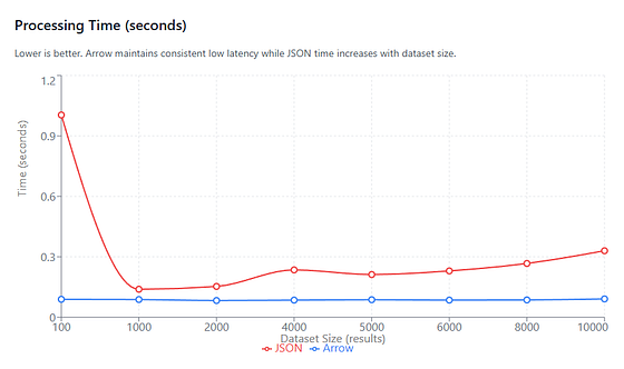
Processing Time (in seconds) vs. Dataset size (number of results). Arrow remains a constant low latency throughout, but using JSON at each stage makes processing time scale with dataset size.
We can ignore the data for very small dataset sizes (that n=100 spike), because then the JSON pipeline appears MUCH slower than it really is due to fixed overheads in the JSON pipeline: repeated json.dumps() / json.loads() calls and Python object allocation dominate runtime.
Arrow’s processing time remains nearly constant (~0.085–0.091 seconds) throughout, so here’s how the Arrow speedup grows with dataset size:
- ~1.6x at 1,000 rows
- ~2–3x between 2,000 and 8,000 rows
- ~3.6x at 10,000 rows
This pattern is expected. The JSON pipeline scales processing time linearly with row count, The Arrow pipeline does not: filtering, sorting, and aggregation run inside native kernels over columnar buffers, so Python never enters the per-element hot path.
Throughput
On average (1,000–10,000 rows), Arrow delivers ~2.6x higher throughput.
Press enter or click to view image in full size
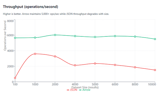
Throughput (operations/second) vs. Dataset size (number of results). Arrow maintains at least 5,000+ ops/sec across all dataset sizes.
Throughput mirrors processing time exactly.
Arrow maintains a relatively constant throughput of ~5,500–6,000 ops/sec across all dataset sizes. The JSON pipeline’s throughput degrades steadily as row count increases, dropping from ~3,600 ops/sec @ 1,000 rows to ~1,500 ops/sec @ 10,000 rows.
Memory Usage (Python Heap)
On average (1,000–10,000 rows), Arrow uses ~84% less Python heap memory.
Press enter or click to view image in full size

Peak Memory Usage (in MB). Pipelines that use Arrow use 80–100% less memory across all dataset sizes.
Peak memory usage, measured via tracemalloc, shows a consistent and substantial reduction when using Arrow (again, we can ignore the test case with n=103.) Bear in mind we’re capturing Python heap allocations only.
As dataset size increases, JSON memory usage remains tied to object churn, while Arrow’s Python-level memory stays low and stable — most data lives in native buffers outside the Python object model.
File Size (JSON vs Parquet)
On average (1,000–10,000 rows), Parquet files are ~98.7% smaller than JSON.
Press enter or click to view image in full size
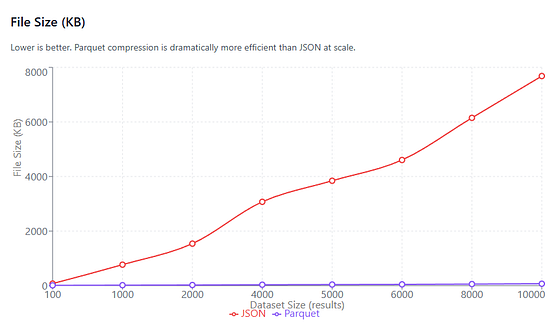
File Size (in KB) vs. Dataset size (number of results). Arrow based pipelines compress persisted results dramatically better than pipelines which use JSON.
The most dramatic — but also the most boringly predictable difference.
Parquet files are consistently 97–99% smaller than their JSON equivalents at realistic dataset sizes. No surprises there, that’s exactly what columnar formats like Parquet were designed to do.
How Much Money Does This Save You?
Breaking this down:
- ~2.6x faster processing (average) = ~1/2.6th the compute time
- ~84% less Python heap memory = smaller instance sizes, less GC pressure
- ~98–99% smaller files = lower storage and I/O costs
So for a pipeline that processes, say, 10,000 queries/day, a JSON approach would use ~10,000 seconds of compute time while an Arrow approach would use ~3,800 seconds of compute time
Assuming $0.10/hour for compute, that’s ~$0.28/day vs ~$0.11/day — roughly a 60% reduction in compute cost, before even accounting for memory and storage savings. I’ll take that any day.
When Should You Use Apache Arrow?
Here’s the big caveat — you can’t just use Apache Arrow for everything. It is an architectural choice for production data pipelines rather than some general optimization hack.
Use an Arrow-based pipeline when:
- You process dozens to thousands of rows per batch
- Your pipeline applies multiple transformations (e.g. filter → sort → aggregate → export)
- You’re building analytics, feature extraction, or training pipelines
- Memory usage, throughput, or storage size matter
- You might want to persist data in Parquet for downstream systems
Honestly though, from experience, most production data pipelines should find using Arrow a net improvement. In these cases, avoiding that repeated Python object materialization + serialization tax will dramatically improve how your pipeline scales (and how much it costs to operate.)
Keep your existing pipeline when:
- You’re running one-off scripts on very small datasets
- The end of your pipeline has to return JSON directly to another API consumer
- Your data can’t be described by a schema
- You aren’t transforming the data at all (the conversion cost won’t amortize)
Adopting Apache Arrow just won’t be worth the effort (or rewrite) in those cases.
Frequently Asked Questions
Common questions about this topic
What is Apache Arrow?
Apache Arrow is an open-source columnar, in-memory data format that stores each column as a contiguous buffer of typed values instead of representing data as a collection of row objects.
How does Arrow change the execution model compared to parsing JSON into language-native objects?
Arrow moves computation out of the per-row, language object model into operations over contiguous column buffers in native code, so most transformations avoid creating language-level objects and run vectorized, cache-friendly kernels instead of per-element interpreter loops.
What does “zero-copy” mean in the context of Arrow?
“Zero-copy” means avoiding repeated parse/encode cycles and language-level object creation for the hot path; it does not mean no memory is ever allocated, but rather that operations reuse existing buffers and avoid materializing per-row objects repeatedly.
What are the common performance problems caused by using JSON as an interchange format between pipeline stages?
Common problems are per-element execution overhead (one loop, lookup, allocation per row), repeated conversions between JSON and language objects across stages (multiple json.loads/json.dumps), and high memory overhead from row-oriented object graphs where each row and field becomes separate heap objects and pointers.
What typical workflow improvements does switching to Arrow solve?
Switching to Arrow reduces per-element interpreter overhead by running native vectorized operations on columns, eliminates repeated serialize/deserialize cycles between stages, and significantly lowers Python heap memory usage by keeping most data in native buffers.
What benchmarking setup was used to compare JSON and Arrow pipelines?
The benchmark simulated a pipeline that fetches SERP JSON, converts to Arrow once, then repeatedly performs filter, sort, and aggregation operations for many iterations (500), measuring runtime with time and Python heap memory with tracemalloc, and comparing JSON+serialize/deserialize loops versus Arrow-native operations and Parquet file sizes.
What average processing time improvement did the benchmark observe for Arrow?
On average for datasets from about 1,000–10,000 rows, Arrow achieved approximately 2.6x faster processing time compared to the JSON-based pipeline.
What average memory improvement did the benchmark observe for Arrow?
On average for datasets from about 1,000–10,000 rows, Arrow used approximately 84% less Python heap memory as measured with tracemalloc.
How much smaller were persisted Parquet files compared with JSON in the benchmark?
Parquet files were consistently much smaller, roughly 97–99% smaller than equivalent JSON files across realistic dataset sizes in the benchmark.
What example end-to-end savings were reported when switching a daily pipeline from JSON to Arrow?
Using the reported average improvements, a pipeline processing 10,000 queries/day reduced compute time from about 10,000 seconds to about 3,800 seconds, translating in the example to roughly a 60% reduction in compute cost at $0.10/hour before accounting for memory and storage savings.
What project steps and components are required to build the Arrow-based pipeline demonstrated in the benchmark?
The demonstrated pipeline includes: an API client to fetch JSON (optional if JSON already exists), a JSON→Arrow conversion function that defines a schema and builds a pyarrow.Table, Arrow-native transformations (filter, sort, select, aggregate) using pyarrow.compute, and optional export to Parquet via pyarrow.parquet for persistence.
When is using Apache Arrow recommended and when is it not worth the effort?
Use Arrow when processing dozens to thousands of rows per batch, applying multiple transformations (filter→sort→aggregate→export), building analytics/feature-extraction/training pipelines, caring about memory/throughput/storage, or wanting Parquet persistence. Keep the existing JSON pipeline for one-off scripts on very small datasets, when the pipeline must return JSON directly to another API consumer, when data cannot be described by a schema, or when no transformations occur so conversion cost cannot be amortized.
POSTS ACROSS THE NETWORK

Stop Using Express.js in 2026: The Modern Node.js Backend Stack That Replaced It

Next.js App Router vs Pages Router: After 6 Months in Production

Respin Mechanics Explained Through Game State Design
Best 3 Chainguard Alternatives for Hardened Container Images in 2026
Best Stereo Camera for High-Precision 3D Scanning
